Randomized SVD - Randomized Numerical Linear Algebra with Examples

The Randomized SVD is perhaps the most widely known RandNLA algorithm, having been popularized in Halko et al., 2011. This is perhaps to its simplicity and outstanding practical effectiveness.

Note that the output of Algorithm 5.1 can be easily factored into an “SVD-like” form $\vec{U} \vec{\Sigma} \vec{V}^\T$ (where $\vec{U}$ and $\vec{V}$ have orthonormal columns and $\vec{\Sigma}$ is non-negative and diagonal) by computing the SVD $\vec{U}'\vec{\Sigma}\vec{V}^\T = \Call{svd}(\vec{X}^\T)$ and then setting $\vec{U} = \vec{Q}\vec{U}'$ .

The approximation is not necessarily of rank- $k$ . In most cases this is not an issue, but if a rank- $k$ approximation is required, one can simply truncate the approximate SVD to the first $k$ singular values; i.e. output $\vec{Q} \llbracket \vec{X}^\T \rrbracket_k$ .

def randomized_SVD(A,k,b,rank_exactly_k=False):

    n,d = A.shape
    Ω = np.random.randn(d,b)
    Y = A@Ω
    Q,_ = np.linalg.qr(Y,mode='reduced')
    X = A.T@Q
    Up,s,Vt = np.linalg.svd(X.T,full_matrices=False)

    if rank_exactly_k:
        return Q@Up[:,:k],s[:k],Vt[:k]
    else:
        return Q@Up,s,Vt

Numerical Example¶

Let’s load an image as a numpy array. Here the image is of dimension 1333 by 2000.

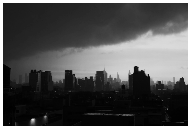
Compression via SVD¶

We can use the SVD to compress the image. When $k\approx 100$ , we see that the resulting image is essentially indistinguishable from the original image. However, by storing the compressed image in factored form, we require just $(n+d)k = 3.3\times 10^{5}$ parameters, which is roughly $12\%$ of the $nd = 2.6\times 10^6$ parameters required to store the original image!

start = time.time()
U,s,Vt = np.linalg.svd(A,full_matrices=False)
end = time.time()

SVD_time = end-start

k = 100 # target rank

plt.imshow(U[:,:k]@np.diag(s[:k])@Vt[:k],cmap='gray')
plt.axis('off')
plt.tight_layout()

Randomized SVD¶

Now let’s consider the Randomized SVD. We’ll use a block size $b=2k$ , and truncate back to rank- $k$ . Similar to the exact SVD, the rank-100 approximation produces by the Randomized SVD looks the same as the original image.

start = time.time()
U_rsvd,s_rsvd,Vt_rsvd = randomized_SVD(A,k,2*k,rank_exactly_k=True)
end = time.time()

RSVD_time = end-start


plt.imshow(U_rsvd@np.diag(s_rsvd)@Vt_rsvd,cmap='gray')
plt.axis('off')
plt.tight_layout()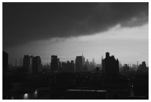

Runtime comparison¶

The upshot is that the Randomized SVD is way faster!! In this case roughly 20 times faster.

timing = [{
    'method':'SVD',
    'time (s)': SVD_time,
    'speedup': 1
},
{
    'method':'Randomized SVD',
    'time (s)': RSVD_time,
    'speedup': SVD_time/RSVD_time
}]

pd.DataFrame(timing).reindex(columns=['method','time (s)','speedup']).style.format({
    'time (s)': '{:.4f}',
    'speedup': '{:.1f}x',
})

Theoretical bounds¶

A prototypical bound for the Randomized SVD is the following:

Bounds for the spectral norm are also available.

Full analyses can be found in Halko et al., 2011Tropp & Webber, 2023, but getting some intuition is pretty simple! Write the SVD of $\vec{A}$ as

\vec{A} = \begin{bmatrix}\vec{U}_1 & \vec{U}_2 \end{bmatrix} \begin{bmatrix} \vec{\Sigma}_1 \\ & \vec{\Sigma}_2 \end{bmatrix} \begin{bmatrix} \vec{V}_1^\T \\ \vec{V}_2^\T \end{bmatrix},

(5.2)

where $\vec{U}_1$ , $\vec{\Sigma}_1$ and $\vec{V}_1$ correspond to the top- $k$ singular vectors of $\vec{A}$ ; i.e. $\llbracket \vec{A} \rrbracket_k = \vec{U}_1 \vec{\Sigma}_1 \vec{V}_1^\T$ .

Observe that

\vec{Y} = \vec{A}\vec{\Omega} = \vec{U}_1\vec{\Sigma}_1\vec{V}_1^\T \vec{\Omega} + \vec{U}_2\vec{\Sigma}_2\vec{V}_2^\T \vec{\Omega}.

(5.3)

In the case that $\vec{\Sigma}_2 = \vec{0}$ , then we will obtain $\vec{Q}$ so that $\range(\vec{Q}) = \range(\vec{U}_1)$ . In this case, $\vec{Q}\vec{Q}^\T$ would be the orthogonal projector onto the top left singular vectors of $\vec{A}$ , and we would recover the best rank- $b$ approximation. However, when $\vec{\Sigma}_2$ is nonzero, then the $\vec{Y}$ we get is perturbed from this ideal case. However, for matrices with fast singular-value decay, $\vec{\Sigma}_2$ will be small, and the impact won’t be so big. Similarly, by increasing $b$ , we can make $\vec{\Sigma}_2$ smaller.

References¶

Halko, N., Martinsson, P. G., & Tropp, J. A. (2011). Finding Structure with Randomness: Probabilistic Algorithms for Constructing Approximate Matrix Decompositions. SIAM Review, 53(2), 217–288. 10.1137/090771806
Tropp, J. A., & Webber, R. J. (2023). Randomized algorithms for low-rank matrix approximation: Design, analysis, and applications. https://arxiv.org/abs/2306.12418

Randomized Numerical Linear Algebra with Examples

Low-Rank Approximation